Analyzing machine code
Our optimization efforts at the heart of the simulation have taken us to the point where we are computing output data points at a pretty high rate compared to what we started with:
run_simulation/128x64/total16384/image1/compute
                        time:   [88.342 ms 88.415 ms 88.469 ms]
                        thrpt:  [1.5171 Gelem/s 1.5180 Gelem/s 1.5193 Gelem/s]

run_simulation/512x256/total1024/image1/compute
                        time:   [83.000 ms 84.254 ms 85.751 ms]
                        thrpt:  [1.5652 Gelem/s 1.5930 Gelem/s 1.6171 Gelem/s]

run_simulation/2048x1024/total64/image1/compute
                        time:   [135.99 ms 138.66 ms 140.84 ms]
                        thrpt:  [952.99 Melem/s 967.97 Melem/s 986.98 Melem/s]

run_simulation/4096x2048/total16/image1/compute
                        time:   [221.10 ms 221.60 ms 222.27 ms] thrpt:  [603.84
                        Melem/s 605.68 Melem/s 607.05 Melem/s]
But there are two questions that we should be asking ourselves right now:
- How far are we from peak hardware performance at small problem scales?
- Why is it the case that performance did not improve as much for the larger problem sizes as it did for the smaller problem sizes?
In this chapter, we will investigate the first question. And in doing so, we will also prepare the way for subsequent chapters, which will answer the second question.
Counting clock cycles
To put the small scale numbers in the perspective of raw hardware capabilities, let’s look into some execution statistics for the 512x256, which performs best at the moment:
$ perf stat cargo bench --bench simulate -- 'run_simulation/512x256/total1024/image1/compute$'

       [ ... benchmark output ... ]

      28 934,68 msec task-clock                       #    1,379 CPUs utilized
         11 660      context-switches                 #  402,977 /sec
          1 076      cpu-migrations                   #   37,187 /sec
        199 617      page-faults                      #    6,899 K/sec
295 945 818 356      instructions                     #    2,44  insn per cycle
                                                      #    0,02  stalled cycles per insn     (80,01%)
121 371 248 616      cycles                           #    4,195 GHz                         (79,98%)
  5 299 370 710      stalled-cycles-frontend          #    4,37% frontend cycles idle        (79,98%)
 22 923 089 669      branches                         #  792,236 M/sec                       (80,03%)
    208 598 966      branch-misses                    #    0,91% of all branches
    (80,00%)
The two most important pieces of information here are that…
- We’re executing more than 2 instructions per clock cycles, which is the maximal execution rate for most CPU instructions (loads, multiplications, FMAs…). This suggests that we manage to execute instructions of different type in parallel, which is good.
- Our average CPU clock rate when executing this benchmark is 4.2 GHz, which when divided by the output production rate tells us that it takes us about about 2.6 CPU clock cycles to produce one output data point.
We also know that this Zen 2 CPU uses AVX vectorization and we work using single-precision floating point operations, which means that we process 256/32 = 8 outputs per inner loop cycle. From this, we can deduce that it takes us 21 clock cycles to produce one output data point.
But is that a lot? A little? To know this, we need to take a look at our workload.
Setting the goal
Let’s take a look at the current version of our simulation loop:
for (win_u, win_v, out_u, out_v) in stencil_iter(start, end) {
    // Access the SIMD data corresponding to the center concentration
    let u = win_u[STENCIL_OFFSET];
    let v = win_v[STENCIL_OFFSET];

    // Compute the diffusion gradient for U and V
    let gradient = |win: ArrayView2<_>| {
        let weight = |i: usize, j: usize| Vector::splat(STENCIL_WEIGHTS[i][j]);
        let mut acc1 = weight(0, 0) * win[[0, 0]];
        let mut acc2 = weight(0, 1) * win[[0, 1]];
        let mut acc3 = weight(0, 2) * win[[0, 2]];
        acc1 = weight(1, 0).mul_add(win[[1, 0]], acc1);
        acc2 = weight(1, 1).mul_add(win[[1, 1]], acc2);
        acc3 = weight(1, 2).mul_add(win[[1, 2]], acc3);
        acc1 = weight(2, 0).mul_add(win[[2, 0]], acc1);
        acc2 = weight(2, 1).mul_add(win[[2, 1]], acc2);
        acc3 = weight(2, 2).mul_add(win[[2, 2]], acc3);
        acc1 + acc2 + acc3
    };
    let full_u = gradient(win_u);
    let full_v = gradient(win_v);

    // Compute SIMD versions of all the float constants that we use
    let diffusion_rate_u = Vector::splat(DIFFUSION_RATE_U);
    let diffusion_rate_v = Vector::splat(DIFFUSION_RATE_V);
    let feedrate = Vector::splat(options.feedrate);
    let killrate = Vector::splat(options.killrate);
    let deltat = Vector::splat(options.deltat);
    let ones = Vector::splat(1.0);

    // Flush overly small values to zero
    fn flush_to_zero<const WIDTH: usize>(x: Simd<f32, WIDTH>) -> Simd<f32, WIDTH>
    where
        LaneCount<WIDTH>: SupportedLaneCount,
    {
        const THRESHOLD: f32 = 1.0e-15;
        x.abs()
            .simd_lt(Simd::splat(THRESHOLD))
            .select(Simd::splat(0.0), x)
    }

    // Compute the output values of u and v
    let uv_square = u * v * v;
    let du = diffusion_rate_u.mul_add(full_u, (ones - u).mul_add(feedrate, -uv_square));
    let dv = diffusion_rate_v.mul_add(full_v, v.mul_add(-(feedrate + killrate), uv_square));
    *out_u = flush_to_zero(du.mul_add(deltat, u));
    *out_v = flush_to_zero(dv.mul_add(deltat, v));
}
If we think about the minimal amount of SIMD processing work that our CPU is doing for each output computation, i.e. the work that is dependent on a particular sequence of inputs and cannot be deduplicated by the compiler across loop iterations, we see that…
- We load 9 input vectors for each species, 9x2 = 18 overall.
- Of these 9x2 inputs, 6x2 are shared with the previous computation due to our sliding window pattern. For example, the central value of a particular input window is the left neighbor of the next input window. But for register pressure reasons that will be covered later in this chapter, the compiler is unlikely to be able to leverage this property in order to avoid memory loads on the vast majority of x86 CPUs.
- We compute 3 multiplications for the diffusion gradient of each species and 2
more in the
uv_squarecomputation, so 3x2 + 2 = 8 multiplications overall. - For each species we compute 6 FMAs within the diffusion gradient, 2 more in
du/dv, and 1 more for the finalu/voutput, so 9x2 = 18 FMAs overall. - We compute two additions for the diffusion gradient of each species and one
subtraction for the
(ones - u)part ofdu. Therefore we expect a total of 5 runtimeADD/SUBoperations. We don’t expect more additions/subtractions/negations, even though the code would suggest that there should be more of them happening, because…- The
-(feedrate + killrate)computation should be automatically extracted from the loop by the compiler because it operates on loop-invariant inputs and always produces the same result. - The negative
-uv_squareaddend in the FMA ofducan be handled by a special form of the x86 FMA instruction calledFMSUB.
- The
- For each
u/voutput we perform a flush-to-zero operation that involves an absolute value, a SIMD comparison and a SIMD masked selection, that’s at least 3x2 = 6 more SIMD operations. - Finally we store 1 output vector for each species, so we have 2 stores overall.
So we know that as a bare minimum, assuming the compiler did everything right, we need to perform 57 SIMD operations to compute an output data point. And if we account for the fact that x86 is a complex instruction set where most arithmetic instructions can also load an input from memory, but FMA cannot store data to memory, we reach the conclusion that these operations cannot be encoded into less than 57-18 = 39 x86 instructions.
There has to be more to the actual compiler-generated code for the inner loop, however, because our simulation has many constant inputs:
- The
STENCIL_WEIGHTSmatrix contains three distinct values:0.25,0.5and-3.0. DIFFUSION_RATE_UandDIFFUSION_RATE_Vare two other distinct constants,0.1and0.05.- We have three runtime-defined parameters whose value is unknown to the
compiler,
feedrate,killrateanddeltat.deltatandfeedrateare used as-is, whilekillrateis used as part of the-(feedrate + killrate)expression. - We need the constant
1.0for the(ones - u)computation. - We need
THRESHOLDand the constant0.0for theflush_to_zerocomputation.
That’s 11 constants, which is a lot for the majority of x86 CPUs that do not implement AVX-512 but only AVX. Indeed, the AVX instruction set only features 16 architectural vector registers and its vector operations only support inputs from memory and these vector registers. Which means that if we keep all constant state listed above resident in registers, we only have 5 registers left for the computation, and that is not a lot when we aim to implement the computation in a manner that exhibits a high degree of instruction-level parallelism.
As a result, compilers will usually not try to keep all of these constant values
resident in registers. They will only keep some of them, and store the other
ones in memory at the start or update(), reloading them on each loop
iteration. This register spilling, as it is called, means that our inner loop
will have more memory loads than it strictly needs by the above definition, in
the name of performing other computations more efficiently using the CPU
registers that this frees up.
Finally, so far we have only focused on the computation of one output data point, but that computation appears within a loop. And managing that loop, in turn, will require more instructions. The minimal number of CPU instructions required to manage a simple 1D loop is a loop counter increment, a comparison that checks if the counter has reached its final value, and a conditional branch that takes us back to the beginning of the loop if we’re not done yet.
We could follow this simple logic in our stencil_iterator() iterator
implementation by tracking an offset from the start of each input and output
dataset, which happens to be the same for both input and output data. And
indeed, an earlier version of stencil_iterator() did just that. But due to
arcane limitations of x86 memory operands, it is surprisingly faster on x86 CPUs
to have a loop that is based on 4 pointers (two input pointers, two output
pointers), that each get incremented on each loop iteration, because this speeds
up the indexing of actual input data later in the diffusion gradient
computation. Which is why stencil_iterator() does that instead.
When all these things are taken into account, it is actually quite impressive
that according to perf stat, our program only executes an average of 21 * 2.44 = 51.24 instructions per output data vector. That is only only 7 CPU
instructions more than the minimum of 39+4+2 = 44 instructions required to
perform the basic computation and manage a loop counter. So we can be quite
confident that the compiler produced rather reasonable machine code for our
computation.
But confidence is not enough when we try to reach peak performance, so let’s
take a deeper look at the hot CPU code path with perf record.
Analyzing execution
Collecting data with perf
We can have perf analyze where CPU cycles are spent using perf record and
perf report:
perf record -- cargo bench --bench simulate -- 'run_simulation/512x256/total1024/image1/compute$' --profile-time=100  \
&& perf report

As you can see, 94% of our CPU time is spent in the AVX + FMA version of the
update() function, as we would expect. The remaining time is spent in other
tasks like copying back top values to the bottom and vice-versa (1.68%), and
nothing else stands out in the CPU profile.
We can then display annotated assembly for the update function using the a
key, and it will highlight the hottest instructions, which will let us easily
locate the inner loop:
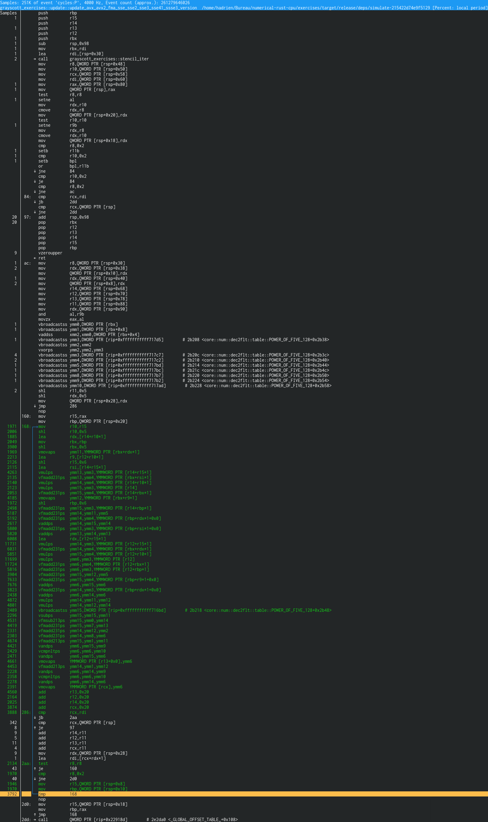
What are we looking at here? Recall that in a nutshell, perf record works by
periodically stopping the program and querying which instruction the CPU is
currently processing. From this information, perf annotate computes a
histogram of assembly instructions where CPU time is most often spent. And what
we are looking at here is this histogram, with color coding added to highlight
the CPU instructions which the program was most often executing at the time
where a sample was taken, which are most likely to be a performance bottleneck.
Now, we should be careful about over-interpreting this data, because “which
instruction the CPU is currently processing” is a trick question on a modern
superscalar, out-of-order and deeply pipelined CPU. perf and the underlying
CPU performance monitoring infrastucture try to avoid producing a biased answer
by using various techniques, such as randomly attributing a particular sample to
any of the instructions that were actively executing at sampling time, but these
techniques not foolproof.
To give two examples…
- Since consecutive pairs of comparison and conditional jump x86 instructions are actually processed as a single operation by the backend of all current x86 CPUs. Thus an imbalance of sample counts attributed to the comparison and jump is to be expected, as the CPU artificially spreads the cycle count between these two instructions.
- When an x86 instruction has a memory operand, it is conversely split in two operations at the backend level, one memory load and one operation that operates from registers. Therefore, it is normal if the measured overhead for this instruction is higher than that of an instruction that has a register operand, because the memory operand does more work.
But overall, we can still get significant mileage out of this data numbers by following the general intuition that if some instructions get a high percentage of samples in a certain region of assembly, it suggests that there are hot instructions around this location in the program binary.
So in the example above, vmulps might not be the actual hottest CPU
instruction, the lea above or the vfmadd231ps below might be the one
instead.
In any case, without getting to the level of fine-grained analysis where the above considerations are a problem, we can rather easily figure out what control flow path is taken by the inner loop of the simulation by following the trail of high sample frequencies:
- We know that every inner loop iteration starts at location
168:, as there is negligible sample coverage before that. - We know that the
jb 2aaconditional branch right after location286:is usually taken, because the assembly after it has only little sample coverage. Which suggests that this assembly belongs to the outer loop over lines of output, not the inner loop over storage cells within a line. Inner loop control flow must continue at location2aa:. - We know that the
je 160conditional branch after location2aa:is rarely if ever taken, because there is no sample coverage for the associated assembly at target location160:. - We know that the
jne 2d0conditional branch coming right after that is rarely if ever taken, because there is no sample coverage at the associated2d0:location. - And then the hot code path reaches a
jmp 168jump instruction that takes us back to the beginning of the hot code path, starting the next inner loop iteration.
Now, there are a couple of worrying things in this control flow which suggests that our unsafe iterator implementation could be improved a little to hint the compiler into generating better code:
- The two never-taken branches suggest that the code performs a check for a
condition that should always be true, especially as they repeatedly test the
value of the
r8register which never changes in the inner loop. In other words, the compiler did not manage to remove or deduplicate a redundant check. - To optimize L1i cache locality, compilers try to make the hottest code path follow a straight line, and to make the exceptional path jump away from this straight line. But here outer loop iterations are on the straight line path, and inner loop iterations jump around it. This will not incur a big performance penalty on modern CPUs, but it does indicate that the compiler did not understand the relative likelihood of the inner and outer loop branches. Which in turn can negatively affect generated code if the compiler takes a gamble based on expected branching frequency that turns out to be wrong.
But so far that’s just a couple suboptimal logic instructions in what is otherwise a sea of SIMD operations, so fixing these little flaws seems unlikely to bring a sizeable performance benefit and we will therefore save that work for a rainy day.
Anyway, given the above control flow analysis, we can extract the assembly that actually gets executed by the inner loop, which boils down to this:
 1971 │168:   mov          r10,r15
 2006 │       shl          r10,0x5
 1885 │       lea          rdx,[r14+r10*1]
 2049 │       mov          rbx,rbp
 3900 │       shl          rbx,0x5
 1969 │       vmovaps      ymm11,YMMWORD PTR [rbx+rdx*1]
 2213 │       lea          r9,[r12+r10*1]
 2126 │       shl          r15,0x6
 2115 │       lea          rsi,[r14+r15*1]
 4263 │       vmulps       ymm13,ymm3,YMMWORD PTR [r14+r15*1]
 2135 │       vfmadd231ps  ymm13,ymm4,YMMWORD PTR [rbx+rsi*1]
 2140 │       vmulps       ymm14,ymm4,YMMWORD PTR [r14+r10*1]
 2123 │       vmulps       ymm15,ymm3,YMMWORD PTR [r14]
 2053 │       vfmadd231ps  ymm15,ymm4,YMMWORD PTR [r14+rbx*1]
 4185 │       vmovaps      ymm12,YMMWORD PTR [rbx+r9*1]
 1972 │       shl          rbp,0x6
 2498 │       vfmadd231ps  ymm15,ymm3,YMMWORD PTR [r14+rbp*1]
 5187 │       vfmadd231ps  ymm14,ymm11,ymm5
 5192 │       vfmadd231ps  ymm14,ymm4,YMMWORD PTR [rbp+rdx*1+0x0]
 2617 │       vaddps       ymm14,ymm15,ymm14
 5800 │       vfmadd231ps  ymm13,ymm3,YMMWORD PTR [rbp+rsi*1+0x0]
 5820 │       vaddps       ymm13,ymm14,ymm13
 6008 │       lea          rdx,[r12+r15*1]
11731 │       vmulps       ymm14,ymm3,YMMWORD PTR [r12+r15*1]
 6031 │       vfmadd231ps  ymm14,ymm4,YMMWORD PTR [rbx+rdx*1]
 5851 │       vmulps       ymm15,ymm4,YMMWORD PTR [r12+r10*1]
11699 │       vmulps       ymm6,ymm3,YMMWORD PTR [r12]
11724 │       vfmadd231ps  ymm6,ymm4,YMMWORD PTR [r12+rbx*1]
 5816 │       vfmadd231ps  ymm6,ymm3,YMMWORD PTR [r12+rbp*1]
 3904 │       vfmadd231ps  ymm15,ymm12,ymm5
 7633 │       vfmadd231ps  ymm15,ymm4,YMMWORD PTR [rbp+r9*1+0x0]
 7676 │       vaddps       ymm6,ymm15,ymm6
 3823 │       vfmadd231ps  ymm14,ymm3,YMMWORD PTR [rbp+rdx*1+0x0]
 2438 │       vaddps       ymm6,ymm14,ymm6
 4872 │       vmulps       ymm14,ymm11,ymm12
 4801 │       vmulps       ymm14,ymm12,ymm14
 2489 │       vbroadcastss ymm15,DWORD PTR [rip+0xfffffffffff716bd]        # 2b218 <core::num::dec2flt::table::POWER_OF_FIVE_128+0x2b48>
 2296 │       vsubps       ymm15,ymm15,ymm11
 4531 │       vfmsub213ps  ymm15,ymm0,ymm14
 4419 │       vfmadd231ps  ymm15,ymm7,ymm13
 2331 │       vfmadd231ps  ymm14,ymm12,ymm2
 2303 │       vfmadd231ps  ymm14,ymm8,ymm6
 4674 │       vfmadd213ps  ymm15,ymm1,ymm11
 4421 │       vandps       ymm6,ymm15,ymm9
 2429 │       vcmpnltps    ymm6,ymm6,ymm10
 2471 │       vandps       ymm6,ymm15,ymm6
 4661 │       vmovaps      YMMWORD PTR [r13+0x0],ymm6
 4453 │       vfmadd213ps  ymm14,ymm1,ymm12
 2228 │       vandps       ymm6,ymm14,ymm9
 2358 │       vcmpnltps    ymm6,ymm6,ymm10
 2278 │       vandps       ymm6,ymm14,ymm6
 2391 │       vmovaps      YMMWORD PTR [rcx],ymm6
 4560 │       add          r13,0x20
 2164 │       add          r12,0x20
 2025 │       add          r14,0x20
 3874 │       add          rcx,0x20
 3888 │286:   cmp          rcx,rdi
      │     ↓ jb           2aa  # Skipped outer loop code path below this...
 2134 │2aa:   test         r8,r8  # ...to get back on the main path
   43 │     ↑ je           160
 1970 │       cmp          r8,0x2
   40 │     ↓ jne          2d0
 1946 │       mov          r15,QWORD PTR [rsp+0x8]
 1970 │       mov          rbp,QWORD PTR [rsp+0x10]
 3792 │     ↑ jmp          168
…and now that we have it, let’s see what useful information we can get out of it.
Analyzing SIMD instructions
If we look at the actual mix of generated assembly instructions compared to our theoretical predictions, we see that…
- As predicted, we have 8 SIMD multiplications.
- 6 of these have a memory operand (easily recognizable as a
YMMWORD PTRassembly argument), which means that they load input data, and that identifies them as initializing the accumulator of one of the ILP streams within the stencil computation. - The other 2 multiplications, which take only register arguments, must by
way of elimination come from the
uv_squarecomputation.
- 6 of these have a memory operand (easily recognizable as a
- As predicted, we have 18 FMA operations.
- Only 10 of them have memory operands, instead of the expected 12 FMAs from
the stencil computation. The reason for this is that the central
uandvvalues are used in multiple places within the computation, and therefore they are loaded by two dedicatedvmovapsinstructions to allow reuse. These instructions can be used for either loading or storing data, those that load data are recognizable by the fact that the target register comes as a first argument and the source memory comes as a second argument. - As also predicted, we have a single
VFMSUB, corresponding to the “addition” of-uv_squarein the computation ofdu. Every other instruction is aVFMADD.
- Only 10 of them have memory operands, instead of the expected 12 FMAs from
the stencil computation. The reason for this is that the central
- As predicted, we have 4 additions and 1 subtraction (the latter of which comes
from the
(ones - u)term of the simulation). - As hoped, our flush-to-zero logic translates into three SIMD instructions:
- A
vandpswhich computes the absolute value of our inputs by performing a logical AND with a precomputed boolean mask where all bits are set except for the IEEE-754 sign bit. Note that this means our computation now depends on one more constant value, further increasing SIMD register pressure… - A
vcmpnltpswhich produces a vector of fake floating-point numbers whose binary representation is set to all-one bits where the first input is not less than the second input, and all-zero bits otherwise. - A
vandpswhich performs a logical AND between this mask vector and the original input, thusly returning zero if the first input is less than the second input. Otherwise the original input value is returned.
- A
- And finally, we have a pair of
vmovapsthat store back the simulation output to memory, which are recognizable by the fact that theirYMMWORD PTRannotated memory operand comes first.
This only leaves one SIMD instructions of unidentified purpose, a
vbroadcastss, which loads a scalar value from memory and puts a copy of it in
each lane of a SIMD register. Its most likely purpose is to load one constant
from memory, which the compiler could not keep in a SIMD register without
sacrificing too much instruction-level parallelism as discussed above.
So far, it looks like the compiler is doing a pretty great job with the SIMD code that we gave it!
Analyzing non-SIMD logic
If we now take a look at the surrounding non-SIMD logic, we first find the basic inner loop iteration logic discussed earlier, based on 4 pointer increments instead of 4 base pointers sharing one single global offset because curiously enough this is faster on x86…
4560 │       add          r13,0x20
2164 │       add          r12,0x20
2025 │       add          r14,0x20
3874 │       add          rcx,0x20
3888 │286:   cmp          rcx,rdi
     │     ↓ jb           2aa
…then the aforementioned pair of useless tests that should be investigated someday…
2134 │2aa:   test         r8,r8
  43 │     ↑ je           160
1970 │       cmp          r8,0x2
  40 │     ↓ jne          2d0
…and then a pair of integer loads from main memory, just before we go back to the top of the loop.
1946 │       mov          r15,QWORD PTR [rsp+0x8]
1970 │       mov          rbp,QWORD PTR [rsp+0x10]
3792 │     ↑ jmp          168
Loads from the stack most frequently originate from the compiler running out of registers and spilling some input values to the stack. But we will check how these values are used later to make sure, because such loads can also come from problems with the compiler’s alias analysis, which means that the compiler feels forced load to reload the same values from memory over and over again even though they haven’t changed, because it fails to prove that they haven’t changed.
If we now look at the top of the loop, we first notice 4 lea instructions,
which abuse the CPU’s addressing units to perform integer computations. This is
something to be vigilant about in x86 assembly, because these operations can
trigger the slow path of the CPU’s addressing unit if they use overly
complicated address calculations. But here they are simply being used to compute
additions, which is as fast as an integer ADD if unnecessarily fancier.
1885 │       lea          rdx,[r14+r10*1]
             # ... other instructions ...
2213 │       lea          r9,[r12+r10*1]
             # ... other instructions ...
2115 │       lea          rsi,[r14+r15*1]
             # ... other instructions ...
6008 │       lea          rdx,[r12+r15*1]
By looking around, we can see that these integer additions are used to work around a limitation of x86 addressing modes:
- The position of an input within a 3x3 window is given by the sum of three values, namely the pointer to the top-left corner of the input window (which we maintain as part of the loop logic), the offset associated with the target row, and the offset associated with the target column.
- But an x86 memory operand can only compute the sum of two values, so we cannot compute the sum of these three values inside of a memory operand.
- However, we can deduplicate some computations because we are fetching multiple values from the same row/column of data in each data stream.
The full proof that this is happening is that…
- Of the 4 pointers
r12,r13,r14andrcxmaintained by the core loop logic, we know thatr13andrcxare the output pointers because they are only used when storing data and (rcx-only) checking if the loop is over. This means thatr12andr14are the pointers to the topleft corner of our U and V input windows (we don’t know which is which). - In
muloperations, which we know from the source code to manipulate data from the first row of each 3x3 window of inputs, we see that the two input pointersr12andr14are used as-is and also summed with two valuesr10andr15that stay the same for input addresses associated with theUandVwindows. This tells us that these values contain the offset of the central and right column of data with respect to the topleft corner of an input window. - Our
leaoperations are identical to the nontrivial address calculations used formuloperations. This tells us that the output of eachlearepresents the memory address of the value at the top of the central or right column of each input window. By combining those with ther12and ther15pointers to the top of the left column, we get a total of 6 pointers that each represent the top of a column within the input window for one chemical species. - Each result from an
leais later summed with two other addends, stored inrbxandrbpas part of an x86 memory operand to produce the input address of two FMA operations. We know that FMAs are used to add values from consecutive rows within a column of inputs, which tells us that these two quantities are row offsets. And indeed the same addends are each used for 6 different FMA address calculations, which makes sense because our U and V input data have the same row offset and we are summing 3 values within each row of each input.
There are also a couple of register-register move instructions. We will explain their purpose later. For now it suffices to say that these instructions are also almost free to process on the CPU backend side. Their only cost is on the CPU frontend side, which in inner loops like this is essentially bypassed by the faster micro-operation cache. So in such a small number, they are highly unlikely to have any measurable impact on our program’s runtime performance.
 1971 │168:   mov          r10,r15
              # ... other instructions ...
 2049 │       mov          rbx,rbp
And finally, we have some bitshift instructions, which perform the equivalent of multiplying the number stored inside of a register by 32 or 64, but faster…
 2006 │       shl          r10,0x5
              # ... other instructions ...
 3900 │       shl          rbx,0x5
              # ... other instructions ...
 2126 │       shl          r15,0x6
              # ... other instructions ...
 1972 │       shl          rbp,0x6
…but those are a little more worrying to see around because they come from those ugly memory loads that we mentioned earlier.
For example, if we take the last integer load from the loop…
1970 │ mov rbp,QWORD PTR [rsp+0x10]
…a copy of it is multiplied by 32…
 2049 │       mov          rbx,rbp
             # ... other instructions ...
 3900 │       shl          rbx,0x5
…while the original value is multiplied by 64…
1972 │ shl rbp,0x6
…and this gives us the rbx and rbp row offsets that are later used as the
center and bottom row offsets of all input address calculations (see above).
Similarly, if we take previous integer load at the end of the loop…
1946 │ mov r15,QWORD PTR [rsp+0x8]
…a copy of it is multiplied by 32…
 1971 │168:   mov          r10,r15
              # ... other instructions ...
 2006 │       shl          r10,0x5
…while the original value is multiplied by 64…
2126 │ shl r15,0x6
…and this gives us the r10 and r15 column offsets that are later used as
the center and right column offsets of all input address calculations (see
above).
The reason why it is worrying to see this code is that the compiler should not be computing these offsets on every loop iteration. It should compute them once and reuse them across all iterations.
If the compiler does not manage to do this, it means that it failed to prove
that the row/column stride of the input ArrayViews does not change between
loop iterations. And as a result, the generated code has to keep doing the
following…
- Load the array row/column stride, which
ndarraycounts as a number of elements - Multiply it by the element size, which is 32 bytes for AVX SIMD vectors, to get offset or each row/column of the 3x3 input window in bytes.
- Multiply the same stride by 64, which is two times the element size, to get the offset between the first and last row/column in bytes.
Isn’t there a way we could do better?
Fixing the problem
All of the above actually happens due to a tiny instruction at the top of the
assembly snippet, which is not exercised a lot by the CPU and therefore not
highlighted by perf annotate:
2 │ → call grayscott_exercises::stencil_iter
Even though this code is not called often, the presence of this instruction
means that the Rust compiler did not inline the constructor of our custom
iterator into the update() function, and therefore had to perform some
optimization passes without knowing what this function does.
As a result, the compiler’s optimization passes did not know the initial state of the iterator as perfectly as it could have, and because of this they had to take some pessimistic assumptions, resulting in the poor code generation discussed above.
The author of this course tried to warn the compiler about the danger of not
inlining iterator code by the #[inline] directive, which increases the
compiler’s tendency to inline a particular function…
#[inline]  // <- This should have helped
fn stencil_iter<'data, const SIMD_WIDTH: usize>(
    // [ ... ]
…but alas, the compiler did not take this gentle hint. So we are going to need to switch to a less gentle hint instead:
#[inline(always)]  // <- This is guaranteed to help
fn stencil_iter<'data, const SIMD_WIDTH: usize>(
    // [ ... ]
With this single line change, we get much more optimal generated code, which contains exactly 6 non-SIMD instructions on the inner loop path: 4 pointer additions and one end-of-loop comparison + branch duo. That’s the way it should be.
Exercise
Implement this optimization and measure its performance impact on your machine. You should not expect a huge benefit because we are not bottlenecked by these integer operations, but it should still be a nice little performance boost worth taking.